August 2022: 31°C – 59,2% August 2023: 31°C – 57% Medium temperatures are the same, and -5% Relative Humidity: in these months there aren’t #ENSO influences.
Dott. Alessio Brancaccio, tecnico ambientale Università di L’Aquila, membro partecipante ordinario Fondazione Michele Scarponi Onlus, ideologo ed attivista del movimento ambientalista italiano Ultima Generazione A22 Network
(LaPresse) Una ondata di caldo sta investendo il Mediterraneo orientale e anche la Giordania è coinvolta. Domenica per il secondo giorno clima torrido nel paese con le strade della capitale Amman semideserte ei turisti affaticati dall’afa che si rinfrescano con bibite ghiacciate. Le temperature sono di 10 gradi superiori alla media stagionale e nei prossimi giorni supereranno i 40 gradi.
Dott. Alessio Brancaccio, tecnico ambientale Università degli Studi di L’Aquila, ideologo e consulente tecnico movimento ambientalista Ultima Generazione A22 Network e membro attivo della Fondazione Michele Scarponi Onlus
La notizia è di quelle importanti: El Niño sta per tornare ancora più forte. Il prossimo Autunno potrebbe dunque essere stravolto in quanto gli effetti dei cambiamenti climatici in atto si andranno a sommare a questo particolare fenomeno.
Ma di cosa si tratta e perché è così importante? Il nome un po’ “buffo” El Niño significa “il bambino” in spagnolo: infatti, l’anomalia termica raggiunge in genere il suo apice verso il periodo del Santo Natale, ovvero proprio quello della Nascita del Bambin Gesù. La voce è in spagnolo perché tocca regioni a lingua ispanica dopo la colonizzazione colombiana. Si tratta di un fenomeno su larga scala, osservato sulla superficie dell’Oceano Pacifico tropicale, centrale e orientale e capace di influenzare le condizioni meteo-climatiche globali.
Gli esperti chiamano questa variazione ENSO (El Niño-Southern Oscillation). I cicli che caratterizzano questo fenomeno hanno una durata che va dai 2 ai 6/7 anni circa. La Niña ed El Niño sono rispettivamente un raffreddamento e riscaldamento della superficie oceanica. Durante un episodio di Niña, le acque risultano di 1/3 gradi più fredde del normale, mentre nelle fasi di Niño sono di 1/3 gradi più calde. L’anomalia più preoccupante riguarda proprio questo aspetto: negli ultimi due anni è stata La Niña a dominare la scena a livello planetario e, secondo lo schema classico, le temperature a livello globale sarebbero dovute calare. Ed invece è successo il contrario, il 2022 è stato l’anno più caldo di sempre da quando si registrano i dati meteo e la prima parte dell’Estate 2023 ha fatto registrare valori record (specie a Luglio) con punte fino a 48°C anche in Italia. Questo fatto porta a una riflessione per nulla banale: il riscaldamento climatico in atto, provocato in parte anche dalle attività antropiche, gioca ormai un ruolo così importante da annullare gli effetti di questi immensi meccanismi climatici.
Ma la domanda sorge spontanea: cosa accadrà quando gli effetti del global warming (riscaldamento globale) si andranno a sommare con quelli di El Niño? Intanto, quello che sappiamo è che la NOAA, l’agenzia statunitense che si occupa di dinamiche oceaniche ed atmosferiche, ha appena annunciato che le acque superficiali dell’Oceano Pacifico si stanno scaldando oltre le aspettative e quindi El Niño è più che confermato. La mappa qui sotto conferma questa anomalia con i valori che si porteranno ben sopra le media climatiche (colore rosso in pieno oceano, davanti alle coste del Sud America).
Riscaldamento delle acque superficiali delle acque del Pacifico (colore rosso)
Stiamo parlando di un fenomeno che riguarda una superficie vastissima, praticamente tutto l’intero Oceano Pacifico.
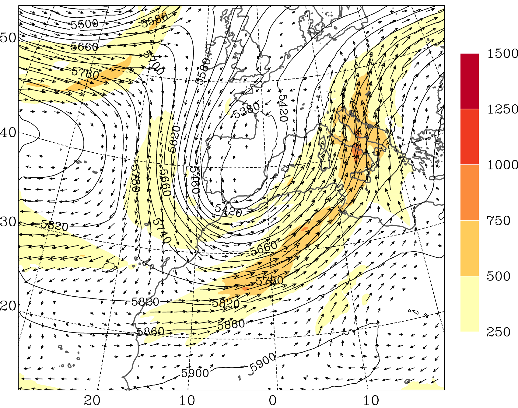
In caso di eventi “forti” di El Niño possono esserci ripercussioni indirette anche sul clima d’Europa. Anomalie positive molto elevate di temperatura sul Pacifico nord-orientale favoriscono lo sviluppo dei cosiddetti “fiumi troposferici”, cioè enormi quantitativi di calore latente che dall’Oceano si trasferiscono all’atmosfera, salendo fino ad alta quota.
Questi fiumi di aria calda una volta saliti tendono a ridiscendere verso il basso nelle zone subtropicali, alimentando i grandi anticicloni permanenti come l’alta pressione delle Azzorre o l’alta pressione africana. Di conseguenza è lecito attendersi anche nella prossima stagione una maggiore spinta dell’anticiclone africano verso il bacino del Mediterraneo con valori termici ben sopra le medie climatiche di riferimento. Attenzione però, il caldo intenso influenza anche la temperatura dei mari, con valori che si sono già portati intorno ai 28/30°C su buona parte dei bacini: stiamo parlando di un’anomalia di circa 4/5°C oltre le medie di riferimento. Tutto ciò si traduce in una maggior energia potenziale in gioco, ovvero quel carburante necessario per lo sviluppo di fenomeni estremi anche per i prossimi mesi autunnali.
Queste condizioni, per esempio, potrebbero portare sulle aree meridionali allo sviluppo di Medicane (dalla fusione dei termini inglesi MEDIterranean hurriCANE “uragano mediterraneo”), ossia violente perturbazioni che si formano quando una bassa pressione viene alimentata dalle acque calde del Mediterraneo e sviluppa caratteristiche da tempesta tropicale. Anche se spesso hanno breve durata, i Medicane possono portare forti piogge e forti raffiche di vento fino a oltre i 120 km/h.
Insomma la prossima stagione rischia di essere molto movimentata sul fronte atmosferico, non resta che seguire passo passo gli aggiornamenti per capire meglio l’evoluzione e che tipo di effetti aspettarci alle nostre latitudini con l’arrivo ormai imminente de El Niño.
Dott. Alessio Brancaccio, tecnico ambientale Università di L’Aquila, membro partecipante ordinario Fondazione Michele Scarponi Onlus, ideologo ed attivista del movimento ambientalista italiano Ultima Generazione A22 Network
Questo secondo un recente studio, anche se diversi scienziati non concordano del tutto con questa previsione. Certo è che la sua intensità sta diminuendo nel corso degli anni
Il costante aumento delle temperature globali sta causando una riduzione nell’intensità della corrente del Golfo, il cui completo arresto avrebbe enormi conseguenze sul clima del Pianeta. I risultati di uno studio appena pubblicato su Nature Communications indicano che questo potrebbe accadere addirittura nel corso di questo secolo, anche se non tutta la comunità scientifica concorda con questa previsione. Una cosa è certa: è necessario, anzi, urgente, ridurre le emissioni di CO2 per tentare di invertire la rotta nell’innalzamento delle temperature globali.
Il “motore” della corrente del Golfo
Gli oceani e le correnti al loro interno giocano un ruolo fondamentale nel mantenere una certa stabilità climatica: la corrente del Golfo, ad esempio, consente la redistribuzione di calore dalle zone tropicali verso i poli. Infatti, spiega la Nasa, questa corrente si sposta lungo la costa orientale del Nord America, rilasciando lungo il suo viaggio parte del calore accumulato ai tropici. Infatti, al suo arresto conseguirebbe, fra le altre cose, una drastica riduzione delle temperature in Europa. Ma qual è il “motore” di questa corrente? In sostanza, la sua esistenza dipende da due fattori: la temperatura e il grado di salinità dell’acqua. L’acqua fredda e salata è più densa di quella calda e contenente una minore quantità di sale disciolto al suo interno. Questo fa sì che in alcune zone dell’oceano si creino le condizioni giuste affinché l’acqua superficiale, una volta che ha rilasciato nell’aria una quantità sufficiente di calore ed è quindi diventata meno densa, si insinui nelle profondità “lasciando spazio” alla corrente calda del Golfo, che prenderà il suo posto. Questo fenomeno fisico garantisce il ciclico movimento delle acque che, come dicevamo, contribuisce a mantenere il clima che conosciamo nelle varie zone del Pianeta.
Oceani e cambiamento climatico
Il cambiamento climatico dovuto alle emissioni di CO2 incide in due modi (collegati fra loro) su questo fenomeno: in primis, sia la temperatura dell’aria che quella dell’oceano stanno globalmente aumentando, riducendo la capacità delle correnti (troppo calde e quindi poco dense) di inabissarsi in profondità. L’aumento delle temperature globali causa contemporaneamente lo scioglimento dei ghiacciai della Groenlandia: questo fa sì che una grande quantità di acqua dolce venga riversata nell’oceano, riducendone la concentrazione salina e quindi, di nuovo, la densità. In buona sostanza, si sta progressivamente riducendo la quantità di acqua “pronta” ad inabissarsi, fenomeno da cui dipende appunto l’esistenza della corrente del Golfo. Le evidenze del fatto che la sua intensità si stia riducendo nel corso degli anni sono ormai diverse. La domanda cruciale è quanto tempo rimane prima che la corrente si fermi del tutto.
Opinioni discordanti
Secondo l’ultimo report dell’Ipcc(Intergovernmental Panel on Climate Change), un completo collasso entro la fine di questo secolo è relativamente improbabile, nonostante gli evidenti segnali di rallentamento. Di diversa opinione sono invece i due autori del recente articolo, che, utilizzando calcoli statistici e i dati relativi alle temperature dell’oceano registrate negli ultimi 150 anni, prevedono che il completo arresto della corrente del Golfo potrebbe verificarsi fra il 2025 e il 2095, con probabilità massima attorno al 2057.
Come riporta una news di LiveScience, altri esperti sostengono che alcune assunzioni incluse nei modelli utilizzati per giungere a tale conclusione siano in realtà troppo semplicistiche, o comunque necessitino di ulteriori verifiche. Ma al di là di stabilire una data esatta, questione su cui gli scienziati continueranno a lavorare, resta valido l’appello del primo autore dello studio Peter Ditlevsen, professore presso il Niels Bohr Institute (Danimarca): “I nostri risultati sottolineano l’importanza di ridurre le emissioni globali di gas serra il prima possibile”.
The Northwest Atlantic Shelf provides ecological and economic benefits along the heavily populated North American coastline and beyond. In 2009-2010, abrupt warming prompted an ecosystem shift with consequences for fisheries, yet the cause of this event is unclear. Here we use satellite altimetry and in situ measurements to show that, in 2008, the Gulf Stream migrated closer to the Tail of the Grand Banks, a shift that has persisted ever since. This change reduced the westward connectivity of the Labrador Current that otherwise supplies cold, fresh, oxygen-rich waters to the shelf. Within one year after the appearance of anomalously warm and saline water at the Tail of Grand Banks, subsurface warming progressed south-westwards. Historical observations suggest a similar sequence of events may have occurred in the 1970s. Therefore, monitoring water properties at the Tail of Grand Banks may offer predictability for shelf properties and ecosystem perturbations with substantial lead time.
Introduction
The Northwest Atlantic Shelf is among the fastest warming regions in the global ocean1 (Fig. 1). This region is home to ecologically and economically valuable marine species, including the American lobster and the Atlantic sea scallop—two of the most valuable single-species fisheries in the United States2. The Northwest Atlantic surface warming during at least the past 4 decades has been attributed to both natural and anthropogenic forcing3, and has been enhanced in recent years by atmospherically driven extreme events4,5. Shelf bottom waters have also warmed in recent decades, but with distinct temporal and spatial patterns when compared to the surface warming, suggesting that different forcing factors are likely at play here6. In one high-resolution model, simulated warming events in the Northwest Atlantic are strongly correlated with negative anomalies in the strength of the Atlantic Meridional Overturning Circulation (AMOC), leading to the interpretation that recent and historic warming in this region is an indicator of AMOC slowing in the 20th century7. Under continuous greenhouse gas emissions, the AMOC slowdown and the associated warming of the Northwest Atlantic8 are expected to increasingly alter historically exploited stocks in this region, demanding adaptation of fisheries risk assessments to maintain resilience in a changing climate9,10.
The red (blue) shading indicates warming (cooling) of the vertically averaged ocean temperature from the EN4 objective analysis to 2000 m, or the seafloor if it is shallower than 2000 m, in 0.5 °C increments (change in the unshaded region is between −0.25 and 0.25 °C). Background in grayscale shows the bathymetry of the region, with darker shades representing shallower areas. The main circulation features that influence the shelf properties are associated with the Gulf Stream (red) and the Labrador Current (blue) systems, as depicted with arrows. The purple arrows show the waters entering the Gulf of Maine are influenced by both current systems. Coastal and shelf areas of interest are indicated. TGB = Tail of the Grand Banks.
The Northwest Atlantic is also the locale where the swift, deep-reaching Gulf Stream and Labrador Current are in close proximity, as they transport warm, salty subtropical water poleward and cold, fresh Labrador Sea Water equatorward, respectively (see schematized currents in Fig. 1). In this region, some of the longest continuous records of ocean temperature and salinity have been collected, several dating to before the turn of the 20th century. More than 50 years ago, these records had already revealed that the sea surface temperature could fluctuate by up to 2 °C on a decadal timescale over a region extending at least from the coast of New Jersey, US to Halifax, Canada11. Subsequent research linked these temperature fluctuations to ripples through the food web and fisheries1,12,13,14,15,16, and showed that one of their drivers may be a modulation in the westward transport of the Labrador Current south of the shallow underwater plateau known as the Grand Banks of Newfoundland17,18,19 (see Fig. 1 for currents and landmarks).
More recently, a high-resolution model simulation suggested that the decreasing proportion of Labrador Current water on the Northwest Atlantic Shelf coincides with a deepening thermocline at the crossroads of the subtropical and subpolar circulation at the Tail of the Grand Banks (TGB)20. Despite the long history of observations and these more recent model results, a description of the mechanisms involved in the rapid warming of the Northwest Atlantic Continental Shelf has been lacking, hindering our ability to predict these changes in advance. Here we connect abrupt migrations in the Gulf Stream position to the warming of the Northwest Atlantic Shelf and provide an observation-based assessment of the predictability of shelf property changes. Such predictability may ultimately improve forecasts of ecosystem changes in this region.
Results and discussion
Sea level shift at the Tail of the Grand Banks
The strength and position of the Gulf Stream and Labrador Current can be tracked via satellite observations of sea surface height (SSH). The Gulf Stream Extension, with the 25 cm SSH contour marking its axis21,22,23, approaches the TGB as a freely meandering jet at 50°W and, on average, aligns with the 4000-m isobath south of the TGB (Fig. 2a). The Gulf Stream can impinge on the slope at the edge of the TGB, thus increasing the SSH inshore of the 4000-m isobath, or meander away from it. Therefore, to evaluate the presence of the Gulf Stream at the TGB, we quantify the SSH variability in the area inshore of the 4000-m isobath (Fig. 2c). In the summer of 2008, a shift toward higher SSH suggests that the Gulf Stream migrated to a position closer to the TGB. This shift has persisted for more than a decade, with an increase in the mean SSH of 10.8 cm for 2009–2018 as compared to 1993–2007, detected beyond the 95% confidence level via change-point analysis (Supplementary Fig. 1; see “Methods”). Accordingly, the Grand Banks has experienced anomalously high sea levels since 2009.
a Mean dynamic topography (MDT) in the Northwest Atlantic between 1993 and 2018. The thick red contour is the 500-m isobath between 76°W and 48°W, along which the along-slope surface velocities displayed in Fig. 3a are calculated. The black dotted lines indicate the main cross-slope channels in the region: Great South Channel (GSCh), Northeast Channel (NECh), and Laurentian Channel (LCh). The 100-m, 1000-m, 3000-m, and 4000-m isobaths are contoured in gray. b Sea surface height (SSH) difference between 2009–2018 and 1993–2007. To emphasize spatial patterns, the SSH increase averaged over the entire region that is plotted (equal to 4.5 cm) has been subtracted. c Time series of the monthly SSH (dark gray line) and seasonal AutoRegressive Integrated Moving Average (ARIMA) model jointly fit with a change point (light gray line, estimated as described in the “Methods” section) at the Tail of the Grand Banks (i.e., averaged within the thick black contour in panel (a). The blue and red horizontal lines indicate the averaged SSH of −10.5 and 0.3 cm before and after the shift, respectively, in July of 2008. Colormaps in panels (a) and (b) are from the Cmocean package59.
We searched for and quantified the SSH change point specifically at the TGB because the Labrador Current and Gulf Stream are known to interact at this bathymetric feature24. The difference in average SSH before and after 2008 shows a dipole pattern with large positive anomalies along and just shoreward of the 4000-m isobath at the TGB, and negative anomalies in deeper waters (Fig. 2b). Although the dipole-like structure is strongest just offshore of the TGB, it extends as far west as the New England Seamounts along the overall (1993–2018) mean axis of the Gulf Stream. This pattern coincides with an increased amplitude in the variability of the Gulf Stream North Wall position east of 50°W after 2005 (Ref. 25), an increase in the frequency of Gulf Stream deep cyclones after 2008 (Ref. 23), and is consistent with evidence that the Gulf Stream’s path and speed have significantly changed to the east of the New England Seamounts during the altimetry era26,27. In contrast, the SSH and the depth-integrated water temperature north of the Grand Banks along the Labrador Current show no difference between the period before and after the shift, despite the observed sea surface warming in this region3. In other words, neither water column temperature (Fig. 1) nor SSH (Fig. 2b) indicate that changes at the TGB are driven by changes in the Labrador Current from the Labrador Sea to Flemish Cap.
Temperature anomalies on the Northwest Atlantic Shelf
The presence of the Gulf Stream at the TGB has consequences for the continuity of the Labrador Current west of the Grand Banks. The Labrador Current originates as a western boundary current at the edge of the Labrador shelf and flows southward along the Newfoundland shelf break and through the Flemish Pass before it reaches the TGB. At the TGB, the current bifurcates and some of its volume is transported northeastward inshore of the North Atlantic Current28 at an estimated rate as large as 2.6 Sv29,30. The remainder continues to follow the shelf break west of the Grand Banks as the Shelf Break Jet and can still be seen at the Northeast Channel of the Gulf of Maine17,31, as schematized in Fig. 1. At the ocean’s surface, the current speed along the shelf break can be estimated from the gradient of the SSH field across the shelf break (Supplementary Fig. 2), assuming geostrophic balance. Here, we use satellite altimetry to estimate the variability of the Shelf Break Jet along the 500-m isobath between Flemish Pass and Cape Hatteras. The 500-m isobath was chosen because it is the shallowest isobath (in multiples of 100 m) that continuously follows the shelf break between Flemish Pass and Cape Hatteras (i.e., this isobath does not enter the Gulf of St. Lawrence or the Gulf of Maine). Anomalies in the Shelf Break Jet velocity are significantly correlated with the velocity anomalies at the TGB over a distance of more than 2000 km and at lag times consistent with the advective speed of the Shelf Break Jet (Fig. 3a). The signal continuity persists to the southwest beyond the Laurentian Channel and the Northeast Channel of the Gulf of Maine, only breaking down at the Great South Channel. In contrast, Labrador Current anomalies north of the TGB are uncorrelated with velocity anomalies at the TGB and farther to the southwest, further suggesting that the circulation variability along the Northwest Atlantic Shelf break originates at the TGB and not in the Labrador Sea.
a The correlation coefficient between the deseasonalized along-slope surface velocity at the Tail of the Grand Banks of Newfoundland (along the 500-m isobath, at 42°51ʹN, 50°40ʹW) and the deseasonalized along-slope surface velocity downstream toward the Northwest Atlantic Shelf (i.e., along the red line in Fig. 2a) as a function of time lags and distance from the Tail of the Grand Banks. White contours represent the 95% significance level. The dashed black line represents a propagation speed of 130 km month−1 (5 cm s−1). b Map of change-point timing of the 149-m temperature in the Northwest Atlantic. The shades only show grid points whose single change point during 1993–2018 occurred between January/2009 and December/2011. The temperature changes, in °C, associated with these shifts are displayed in Supplementary Fig. 3. Colors are displayed in 3-month intervals. The various hatch marks indicate the grid points used to calculate the regional lagged correlations shown in Table 1: Laurentian Channel (white circles), Scotian Shelf (black plus signs), Gulf of Maine (white triangles) and Mid-Atlantic Bight (black x-marks). The 100-m, 1000-m, 3000-m, and 4000-m isobaths are contoured in gray. The main cross-shelf features are identified. TGB = Tail of the Grand Banks; LCh = Laurentian Channel; NECh = Northeast Channel; GSCh = Great South Channel; CH = Cape Hatteras. Colormaps are from the Crameri package60.
The significant lagged correlations in Fig. 3a provide a means of quantifying the downstream propagation speed of anomalies originating at the TGB. A velocity anomaly along the shelf break takes, on average, nearly 1 year to reach the Great South Channel, which means that it propagates at about 130 km month−1 (or 5 cm s−1). Given that (1) higher SSH at the TGB is associated with lower velocities along the shelf break west of the Grand Banks of Newfoundland, and that (2) the SSH at the TGB has been at a higher state since July of 2008, we expect a decrease in the supply of relatively cold/fresh Labrador waters to the shelf and slope following this shift.
Indeed, temperatures on the Northwest Atlantic Shelf apparently responded to the abrupt sea level increase at the TGB in the summer of 2008, as indicated by strong column-integrated warming (color contours in Fig. 1; see also Supplementary Fig. 3). The timing of the warming on the shelf depends on its proximity to the TGB, as expected from the propagation timescale of the velocity anomalies along the shelf break. Change-point analysis reveals that subsurface warming occurs at increasing lag with distance from the TGB (Fig. 3b), a result that is robust for all depths between 100 and 200 m (Supplementary Fig. 4). In the spring of 2009, the Laurentian Channel experienced the onset of high temperature anomalies that have persisted through the end of our analysis (December 2018). By the summer of 2009, the warming reached the slope and shelf offshore of the Gulf of Maine. In subsequent months, the warm subsurface waters were swept into the Gulf of Maine through the continuous inflow on the northwest side of the Northeast Channel32. The magnitude of the subsurface warming reached 2.5 °C in the Laurentian Channel and exceeded 1 °C in most of the Gulf of Maine (Supplementary Fig. 3). By the end of 2010, warmer subsurface waters enveloped the entire Northwest Atlantic Shelf between the Great South Channel and the Laurentian Channel.
In agreement with the observed warming on the shelf, a recent analysis inferred that the proportion of Labrador Slope Water entering the Gulf of Maine has been below average since 2010 (except for 2014) and reached a record low in 2017 and 2019, when essentially all of the Gulf of Maine slope water in the Northeast Channel was Warm Slope Water33. Simultaneously, the Gulf of Maine and George’s Banks experienced rising bottom temperatures6. The increased proportion of Warm Slope Water in the Gulf of Maine at the expense of Labrador Slope Water may reinforce atmospherically driven marine heat waves, like the unprecedented surface warming in the first half of 20124,5.
South of the Great South Channel, the temperature shift is unlikely the direct result of the anomaly propagation from the TGB. In the Mid-Atlantic Bight, the significant warming shift shown in Fig. 3b occurred after a 1-year lag following the warming on the Scotian Shelf, which is 8–10 months longer than if the anomaly propagated to this region at a speed of approximately 5 cm s−1 (the speed of the black dashed line in Fig. 3a). The breakdown of the coherent propagation downstream of the Great South Channel is consistent with a water mass analysis31 that showed a strong discontinuity in mean temperature and salinity, with a much warmer and saltier shelf break front along the Mid-Atlantic Bight, likely influenced by its close proximity to the Gulf Stream. This discontinuity suggests that other ocean processes likely influence subsurface temperature fluctuations here. For example, the warming after 2011 in this region may be linked to the increased frequency of warm core rings shed by the Gulf Stream and/or northward shifts in the Gulf Stream orientation downstream of the separation point near Cape Hatteras34,35,36, in addition to anomalies in surface heat flux5.
The association of the high SSH anomalies at the TGB and the rapid warming of the Northwest Atlantic Shelf after 2008 was not a one-off event. Between 1993 and 2018, the time series of SSH anomalies at the TGB was significantly correlated at the 99.9% confidence level with the subsurface temperature on the shelf (Table 1; temperatures are averaged over the four regions indicated in Fig. 3c), leading at timescales consistent with the propagation speed of the Labrador Current to the Great South Channel. The progressive lead time of the correlations from the Laurentian Channel (11 months) to the Scotian Shelf (13 months), and Gulf of Maine (14 months) reinforces the westward propagation of temperature anomalies between the Grand Banks and the Northwest Atlantic Shelf. Moreover, the correlations remain significant beyond the 99% level, though smaller in magnitude, at similar lead times after prewhitening (signal shown in Supplementary Fig. 1b). The prewhitening procedure removes all autocorrelation as well as the change point. Thus, the robustness of the correlations to this procedure indicates that the association of SSH anomalies at the TGB and the shelf temperature anomalies is ubiquitous throughout the satellite altimetry era and is not tied only to the 2008 change point or to similarities in seasonal patterns. The association at a lag of about 2 years between the signal at the TGB and the temperature of the Mid-Atlantic Bight is also robust to prewhitening.
The advent of satellite altimetry and the surge in the number of subsurface temperature/salinity measurements on the Northwest Atlantic Shelf in recent decades37,38 shows that the 2008 circulation shift at the TGB likely set off propagating velocity anomalies along the shelf break and shelf warming. Thus, monitoring sea level anomalies at the TGB may help predict impending shelf temperature anomalies with up to a year of lead time. Additionally, the long history of hydrographic surveys in the Northwest Atlantic allows us to place this recent warming event in the context of the long-term variability of subsurface water masses before the satellite altimetry era.
Centennial-scale shelf warming
The TGB has been monitored for iceberg activity since the International Ice Patrol was formed in response to the sinking of the RMS Titanic in 1912 (Ref. 39). As such, it has one of the longest oceanographic records of temperature and salinity anywhere. Here, we look at the historical hydrographic records stretching back nearly a century, to put the 2008 shift in a broader context (Fig. 4). For this purpose, a temperature–salinity (T–S) diagram is useful, as these water properties are conserved beneath the ocean’s surface and change only through mixing. Thus, a T–S diagram reveals the provenance of different water masses (Fig. 4a; see “Methods” for how the 5153 hydrographic and float profiles were analyzed to reduce the influence of temporal variability in sampling on this diagram). For instance, the cold, fresh Labrador Current north of the TGB contrasts strongly with the warm, salty Gulf Stream. All of the decadally averaged T–S profiles at the TGB are within the envelope bounded by the Labrador Current and the Gulf Stream mean profiles in the layers shallower than the Labrador Sea Water.
a Mean decadal profiles of temperature and salinity at the Tail of the Grand Banks between the 1930s and the 2010s are shown as a T–S diagram. The profiles are color-coded by decade of sampling. The blue and red solid lines indicate mean T–S profiles of the Labrador Current and the Gulf Stream, averaged over the blue and red boxes shown in the inset map, respectively. Thin, black lines are the potential density anomalies referenced to the sea surface, with the 27.68 isopycnal (i.e., potential density of 1027.68 kg m−3) and 27.80 isopycnal indicating the upper and lower boundaries of the Labrador Sea Water. A robust locally estimated scatterplot smoothing is applied to the nine decadal profiles at the Tail of the Grand Banks to reduce the effect of outliers at poorly sampled depths. The strategy used to create this diagram while minimizing the influence of variability in the location where the profiles were collected is described in the “Methods” section. b Monthly time series of the 149-m temperature averaged over the Scotian Shelf and Laurentian Channel (grid points marked with black dots in the inset map). Gray shades indicate the error estimate averaged over the respective grid points, calculated as shown in the “Methods” section.
The T–S diagram indicates that the last 10 years are uniquely warm and salty compared to any time in the past 80 years. However, a shift to warmer and saltier water masses in the 1970s was of similar scale to this recent shift, relative to decades that preceded it. This warming and salinification in the 1970s may have been caused by a shift of the Gulf Stream toward the TGB, analogous with the more recent change evidenced from the 2008 rise in SSH (Fig. 2). While the shallower water masses of the thermocline have become warmer and saltier, consistent with more frequent incursions of the Gulf Stream onto the TGB, the temperature and salinity of the deep-water masses, like the Labrador Sea Water, have not changed dramatically or monotonically.
The coldest and freshest decades at the TGB occurred between the 1930s and 1960s, only returning to these conditions briefly in the 1990s. The 1990s were extraordinary in this region for a number of reasons. The wintertime deep convection in the Labrador Sea was the strongest since at least the end of the 1930s40,41, which resulted in the coldest, freshest and thickest Labrador Sea Water layer on record. Anomalously strong wintertime zonal winds in the subpolar North Atlantic in the early 1990s, expressed as a strong, positive North Atlantic Oscillation (NAO) index42, helped drive this convection. This cold period lasted only for the first half of the decade; by the late 1990s, the temperature at the TGB returned to the warmer conditions of the post-1970s (Supplementary Fig. 5).
On the Scotian Shelf and the Laurentian Channel, the subsurface temperatures have followed a similar signal as the TGB over the past 9 decades (Fig. 4b, temperature averaged over the grid points marked with black dots in the inset of Fig. 4a). Between 1930 and 1970, the annual mean subsurface shelf temperatures fluctuated widely, with the 1930s and the 1960s being the coldest decades on record (average ± standard deviation of 7.3 ± 0.9 °C and 7.7 ± 0.9 °C, respectively), separated by an intervening warmer period (1940s–1950s, averaging 8.5 ± 0.9 °C). At the end of the 1960s, rapid warming caused the mean annual shelf temperatures to exceed 9.5 °C for the first time in 1968, a state that persisted with little variation for nearly 40 years (1970s–2000s, averaging 9.1 ± 0.8 °C). In 2009, a second warming event raised the shelf temperature by another 1.6 °C (2010–2018, averaging 10.7 ± 0.7 °C). The subsurface shelf waters since 2012 were warmer than ever previously recorded.
The post-2008 dynamical connection established in Figs. 2 and 3, which links SSH anomalies at the TGB to propagating downstream velocity anomalies and shelf warming, is evident in the TGB T–S time series and Scotian Shelf temperatures (Fig. 4). We speculate that similar dynamics were operating earlier in the 20th century, when the appearance of warm and salty waters at the TGB in the 1970s coincides with warming all along the Northwest Atlantic Shelf. It is unclear if this earlier shift was part of a multidecadal oscillation, yet it is notable that only during the high NAO of the early 1990s did the Scotian Shelf or TGB experience a period nearly as cool or fresh as the 1930s–1960s, and the warming after 2008 started from this warmer baseline.
Conclusions
In this study, satellite-based and in situ observations show the influence of the Gulf Stream on the supply of cold, fresh waters from the Labrador Sea to the Northwest Atlantic Shelf. A heightened presence of the Gulf Stream at the TGB after 2008, revealed by a significant warming (Fig. 1), salinification (Fig. 4), and an increase in SSH (Fig. 2), was associated with subsurface warming along the continental shelf and slope between Nova Scotia and Cape Hatteras after 2009 (Fig. 3b, Supplementary Figs. 3 and 6, and Table 1). The more frequent impingements of the Gulf Stream at the Tail of the Grand Banks limited the advective connection of the Labrador Current along the edge of the Northwest Atlantic Shelf, thereby reducing the supply of cold, fresh and oxygen-rich waters to the shelf. This perturbation caused anomalies to propagate along the slope and arrive at the Gulf of Maine nearly 1 year after the appearance of anomalous properties at the TGB.
Additionally, our analysis of nearly a century of hydrographic data suggests that a similar shift toward more subtropical water at the TGB was linked to shelf warming at the end of the 1960s, from which the system had never fully recovered. This long-term record lends support to the hypothesis, based largely on climate modeling, of a 20th century slowdown in the AMOC, which is correlated with the warming of the Northwest Atlantic Shelf7 and associated with a northward shift of the Gulf Stream and retreat of the Labrador Current8. Idealized models predict a northward migration of the Gulf Stream accompanying AMOC slowdowns43, in line with our observation of the Gulf Stream increasingly impinging on the TGB during shelf warming. In fact, the TGB has been called the “pacemaker” region for the AMOC, and simple dynamical arguments call for AMOC slowdowns to be accompanied by SSH increases at this boundary region44, as observed following 2008 and inferred in the late 1960s from our water mass analysis (Fig. 4).
The recent subsurface warming of the Northwest Atlantic Shelf, associated with a dynamic change at the TGB, coincides with unprecedented surface warming1, salinification45, and severe marine heat waves46,47 that have likely contributed to long-noted trends in fisheries1,14,48,49,50. Our findings not only help to interpret the rapid temperature fluctuations on the shelf, they also present an opportunity to enhance predictability of future warming. Accurately simulating Gulf Stream–Labrador Current interactions at the TGB appears to be crucial to reproducing the last century of shelf warming, and, therefore, will likely help govern the future properties in this region. Furthermore, monitoring the impingement of the Gulf Stream at the TGB offers up to 1 year of lead time for warming events on the Northwest Atlantic Shelf, and these predictive capabilities may be valuable for forecasting ecosystem changes of consequence for fisheries management.
Methods
Satellite altimetry
Altimetric data is derived from satellite observations with Topex/Poseidon (1992–2002), Jason I (2001–2012), and Jason II (2008–present) and made freely available through the Copernicus Marine Environment Monitoring Service (CMEMS, https://resources.marine.copernicus.eu/). The monthly 0.25° × 0.25° gridded absolute dynamic topography between January 1993 and December 2018 is used to calculate the mean SSH in the region bounded by 30°N, 60°N and 80°W, 40°W, as well as the SSH differences following the 2008 shift. The SSH time series at the TGB is calculated by averaging the absolute dynamic topography over the region highlighted with a thick black contour in Fig. 2a.
The monthly 0.25° × 0.25° gridded surface geostrophic velocity, calculated from the gradient of the SSH between January 1993 and December 2018 provides a measure of the surface Shelf Break Jet speed. The surface geostrophic velocity is interpolated onto the 500-m isobath between Flemish Pass and Cape Hatteras, as indicated by the red contour in Fig. 2a, using a piecewise linear approximation. At each grid point along the 500-m isobath, the surface geostrophic velocity is decomposed into along-slope and across-slope components, with positive values pointing toward Cape Hatteras (along-slope) and inshore (across-slope). The direction of the along-slope component is estimated based on the angle between one grid point on the contoured isobath and the nearest point downstream (i.e., toward Cape Hatteras). Its magnitude is then calculated by projecting the surface geostrophic velocity vector onto the along-slope direction. Similarly, the magnitude of the across-slope component is calculated by projecting the velocity vector onto the across-slope direction. Supplementary Fig. 2 illustrates the direction and magnitude of the all-time mean surface geostrophic velocity as projected onto these components. The along-slope velocity is considered the surface Shelf Break Jet speed used to calculate the lagged correlations shown in Fig. 3a.
EN4 profiles
Historical hydrographic and float profile data compiled and made freely available by the Met Office Hadley Centre (https://www.metoffice.gov.uk/hadobs/en4/) are used to probe the multidecadal variability of water mass composition at the TGB from the 1930s to the present51. A total of 5153 profiles taken in April, May, or June within the box 41°N–44°N, 48°W–53°W were analyzed (Supplementary Fig. 6 shows the location of the profiles used for each decade). Pre-ARGO profiles have been historically biased toward these months, and this subset represents 51% of all profiles taken in this region. We avoid aliasing seasonal variability in our multidecadal time series by limiting our analysis to a single well-sampled season20. Poor data was removed based on EN4’s quality-control flag system, and only data points with accepted pairs of potential temperature and practical salinity were used. Each profile was linearly interpolated to a maximum of 55 vertical levels, with 5-m resolution in the top 100 m, 25-m resolution above 250 m, 50-m resolution above 1550 m, and 250-m resolution above 2050 m. The maximum depth of the averaged profiles is 2050 m, as less than 2% of the profiles in the region reach greater depths.
To avoid the aliasing of variability in the location where the profiles were collected in the TGB box, we subtract an appropriate gridded all-time mean T–S profile from each individual observation, as follows. The profiles were bin-averaged into 30 boxes of 0.5° latitude × 1° longitude with a terrain-following penalty, λ�, which sets the “effective distance” between the location of each profile and the center of each box, thereby clustering profiles collected at similar isobaths.
EN4 objective analysis
The monthly 1° × 1° objective analysis gridded product with 42 vertical levels51,55, made freely available by the Met Office Hadley Centre (https://www.metoffice.gov.uk/hadobs/en4/), is derived from the hydrographic and float dataset described above. The temperature field at 149 m in the region bounded by 33°N, 50°N and 77°W, 48°W is used in the change-point analysis described below. Here, the period analyzed is January 1993 to December 2018, coincident with the altimetric data. Twelve additional layers between 56 and 235 m were also analyzed to determine the vertical extent of the changes observed at 149 m.
Decadal changes in the 149-m layer are analyzed in the time series extending back to 1930 (Fig. 4b). The authors of the EN4 objective analysis highlight that this dataset should be used with caution in the analysis of long-term trends, because, during periods with few observations, the analyses relax to climatology51. Supplementary Fig. 7 shows that the Northwest Atlantic has been historically well-observed, as the number of profiles is plotted in a 1° × 1° grid. Over 1.3 million profiles were used to build the objective analyses here, most of which were taken on the shelf and slope.
Change-point analysis
The 2008 shift in the 1993–2018 SSH time series at the TGB is characterized using a seasonal AutoRegressive Integrated Moving Average (ARIMA) model, which explains the SSH based on its own past values (i.e., its own lags and lagged observation errors). We jointly fit a seasonal ARIMA with each possible monthly change point, iterating over all months between January 1997 and December 2014. The timing of the SSH shift is selected as the month at which inserting a change point maximizes the model log-likelihood, and its inclusion is verified by comparing the Akaike information criterion (AIC) to a model without a change point. All change-point analyses are conducted in R56 using the “forecast” package57. The orders of the resulting seasonal ARIMA, chosen via stepwise selection using the AIC, were (2,0,0) × (2,0,0)12. These orders indicate that the SSH time series is mean stationary, aside from the jointly fit level shift, with significant autocorrelation at 1-, 2-, 12-, and 24-month lags, as seen in Supplementary Fig. 1b. These lags are consistent with strong month-to-month and seasonal signals. The temporal autocorrelation structure explains 45.8% of the variability in the time series, and the change point explains an additional 24.1%.
Similar to the analysis of the SSH at the TGB, temperature change points between January 1997 and December 2014 on the Northwest Atlantic Shelf are identified jointly with a seasonal ARIMA model, for each 1° × 1° grid cell between 30–60°N and 40–80°W. The maximum orders we allowed for these seasonal ARIMA models are (1,0,1) × (1,1,1)12, chosen under the assumption that the temperature observations 1 month and 1 year prior to a measurement contain all available information for estimation. We also assume that the temperature time series are mean stationary after accounting for any change points, and therefore do not model a non-seasonal integrated process. However, variation in the magnitude of the seasonal cycle is permitted. Candidate temperature change points are selected as those that maximize the 3-month running mean of the model log-likelihood, in order to avoid choosing isolated, sharp peaks in the likelihood function, and are retained if they both reduce the AIC over a model without a change point and occur between the SSH shift at the TGB (July, 2008) and December, 2011. We chose this window to identify only temperature change points that followed the SSH shift at the TGB, considering the time lags associated with the propagation speed of the Labrador Current described in Fig. 3a.
To study the relationship between temperature change points detected in different regions of the Northwest Atlantic Shelf and the SSH shift at the TGB, mean temperature time series are calculated for areas of grid cells exhibiting similar change-point timing (hatch marks in Fig. 3b). To prewhiten the SSH and regional temperature time series, we filter using the SSH seasonal ARIMA model fit, including the change point, using the R package “TSA”58. For both the raw and prewhitened time series, the strength and time lag of the correlations between the SSH at the TGB and the mean temperature of each identified region are evaluated (Table 1).
Data availability
Altimetric data is derived from satellite observations with Topex/Poseidon (1992–2002), Jason I (2001–2012), and Jason II (2008–present) and made freely available through the Copernicus Marine Environment Monitoring Service (CMEMS, data can be accessed here upon registration). The historical hydrographic and float profile data, as well as the derived 1° × 1° monthly objective analyses gridded product, are compiled and made freely available by the Met Office Hadley Centre (data can be accessed here).
Code availability
The MATLAB code written to load and analyze the data and to generate the figures is available at https://github.com/afonsogneto/Matlab. The R codes used in the change-point analysis are referenced in the “Methods” section and listed in the bibliography.
References
Pershing, A. J. et al. Slow adaptation in the face of rapid warming leads to collapse of the Gulf of Maine cod fishery. Science350, 809–812 (2015).ArticleCASGoogle Scholar
National Marine Fisheries Service. Fisheries Economics of the United States 2016 (NOAA, 2018).
Chen, Z. et al. Long‐term SST variability on the Northwest Atlantic continental shelf and slope.Geophys. Res. Lett.47, e2019GL085455 (2020).Google Scholar
Chen, K., Gawarkiewicz, G. G., Lentz, S. J. & Bane, J. M. Diagnosing the warming of the Northeastern U.S. Coastal Ocean in 2012: a linkage between the atmospheric jet stream variability and ocean response. J. Geophys. Res. Oceans119, 218–227 (2014).ArticleGoogle Scholar
Chen, K., Gawarkiewicz, G., Kwon, Y. & Zhang, W. G. The role of atmospheric forcing versus ocean advection during the extreme warming of the Northeast U.S. continental shelf in 2012. J. Geophys. Res. Oceans120, 4324–4339 (2015).ArticleGoogle Scholar
Friedland, K. D. et al. Trends and change points in surface and bottom thermal environments of the US Northeast Continental Shelf Ecosystem. Fish. Oceanogr.29, 396–414 (2020).ArticleGoogle Scholar
Caesar, L., Rahmstorf, S., Robinson, A., Feulner, G. & Saba, V. Observed fingerprint of a weakening Atlantic Ocean overturning circulation. Nature556, 191–196 (2018).ArticleCASGoogle Scholar
Saba, V. S. et al. Enhanced warming of the Northwest Atlantic Ocean under climate change. J. Geophys. Res. Oceans121, 118–132 (2015).ArticleGoogle Scholar
Gaichas, S. K., Link, J. S. & Hare, J. A. A risk-based approach to evaluating northeast US fish community vulnerability to climate change. ICES J. Mar. Sci.71, 2323–2342 (2014).ArticleGoogle Scholar
Hare, J. A. et al. A vulnerability assessment of fish and invertebrates to climate change on the Northeast U.S. Continental Shelf. PLoS ONE11, e0146756 (2016).ArticleCASGoogle Scholar
Lauzier, L. M. Long-term temperature variations in the Scotian Shelf area. ICNAF Spec. Publ.6, 807–816 (1965).Google Scholar
Nye, J. A., Joyce, T. M., Kwon, Y.-O. & Link, J. S. Silver hake tracks changes in Northwest Atlantic circulation. Nat. Commun.2, 412 (2011).ArticleCASGoogle Scholar
Pershing, A. J. et al. Oceanographic responses to climate in the Northwest Atlantic. Oceanography14, 76–82 (2001).ArticleGoogle Scholar
Davis, X. J., Joyce, T. M. & Kwon, Y.-O. Prediction of silver hake distribution on the Northeast U.S. shelf based on the Gulf Stream path index. Cont. Shelf Res.138, 51–64 (2017).ArticleGoogle Scholar
Le Bris, A. et al. Climate vulnerability and resilience in the most valuable North American fishery. Proc. Natl. Acad. Sci. USA.115, 1831–1836 (2018).ArticleCASGoogle Scholar
Schartup, A. T. et al. Climate change and overfishing increase neurotoxicant in marine predators. Nature572, 648–650 (2019).ArticleCASGoogle Scholar
Petrie, B. & Drinkwater, K. Temperature and salinity variability on the Scotian Shelf and in the Gulf of Maine 1945–1990. J. Geophys. Res.98, 20079 (1993).ArticleGoogle Scholar
Gilbert, D., Sundby, B., Gobeil, C., Mucci, A. & Tremblay, G.-H. A seventy-two-year record of diminishing deep-water oxygen in the St. Lawrence estuary: the northwest Atlantic connection. Limnol. Oceanogr.50, 1654–1666 (2005).ArticleCASGoogle Scholar
Brickman, D., Hebert, D. & Wang, Z. Mechanism for the recent ocean warming events on the Scotian Shelf of eastern Canada. Cont. Shelf Res.156, 11–22 (2018).ArticleGoogle Scholar
Claret, M. et al. Rapid coastal deoxygenation due to ocean circulation shift in the northwest Atlantic. Nat. Clim. Change8, 868–872 (2018).ArticleCASGoogle Scholar
Lillibridge, J. L. & Mariano, A. J. A statistical analysis of Gulf Stream variability from 18+ years of altimetry data. Deep Sea Res. II85, 127–146 (2013).ArticleGoogle Scholar
Rossby, T., Flagg, C. N., Donohue, K., Sanchez-Franks, A. & Lillibridge, J. On the long-term stability of Gulf Stream transport based on 20 years of direct measurements. Geophys. Res. Lett.41, 114–120 (2014).ArticleGoogle Scholar
Andres, M. On the recent destabilization of the Gulf Stream path downstream of Cape Hatteras: Gulf Stream path destabilization. Geophys. Res. Lett.43, 9836–9842 (2016).ArticleGoogle Scholar
Rossby, T. On gyre interactions. Deep Sea Res. II46, 139–164 (1999).ArticleGoogle Scholar
Seidov, D., Mishonov, A., Reagan, J. & Parsons, R. Resilience of the Gulf Stream path on decadal and longer timescales. Sci. Rep.9, 11549 (2019).ArticleCASGoogle Scholar
Dong, S., Baringer, M. O. & Goni, G. J. Slow down of the Gulf Stream during 1993–2016. Sci. Rep.9, 6672 (2019).ArticleCASGoogle Scholar
Andres, M., Donohue, K. A. & Toole, J. M. The Gulf Stream’s path and time-averaged velocity structure and transport at 68.5°W and 70.3°W. Deep Sea Res. I156, 103179 (2020).ArticleGoogle Scholar
Rossby, T. The North Atlantic Current and surrounding waters: At the crossroads. Rev. Geophys.34, 463–481 (1996).ArticleGoogle Scholar
Loder, J. W., Petrie, B. & Gawarkiewicz, G. G. The coastal ocean off northeastern North America: a large-scale view. In The Sea, Vol.11 (eds. Robinson, A.R. & Brink, K.H.) 105–133 (Wiley, 1998).
Fratantoni, P. S. & McCartney, M. S. Freshwater export from the Labrador Current to the North Atlantic Current at the Tail of the Grand Banks of Newfoundland. Deep Sea Res. I57, 258–283 (2010).ArticleGoogle Scholar
Fratantoni, P. S. & Pickart, R. S. The western North Atlantic shelfbreak current system in summer. J. Phys. Oceanogr.37, 2509–2533 (2007).ArticleGoogle Scholar
Ramp, S. R., Schlitz, R. J. & Wright, W. R. The deep flow through the Northeast Channel, Gulf of Maine. J. Phys. Oceanogr.15, 1790–1808 (1985).ArticleGoogle Scholar
Northeast Fisheries Science Center. 2020 State of the Ecosystem: New England (NOAA, 2020).
Gawarkiewicz, G. G., Todd, R. E., Plueddemann, A. J., Andres, M. & Manning, J. P. Direct interaction between the Gulf Stream and the shelfbreak south of New England. Sci. Rep.2, 553 (2012).ArticleCASGoogle Scholar
Forsyth, J. S. T., Andres, M. & Gawarkiewicz, G. G. Recent accelerated warming of the continental shelf off New Jersey: observations from the CMVOleander expendable bathythermograph line. J. Geophys. Res. Oceans120, 2370–2384 (2015).ArticleGoogle Scholar
Gangopadhyay, A., Gawarkiewicz, G., Silva, E. N. S., Monim, M. & Clark, J. An observed regime shift in the formation of warm core rings from the Gulf Stream. Sci. Rep.9, 12319 (2019).ArticleCASGoogle Scholar
Toole, J. M., Andres, M., Le Bras, I. A., Joyce, T. M. & McCartney, M. S. Moored observations of the Deep Western Boundary Current in the NWAtlantic: 2004–2014: LINE W 2004–2014. J. Geophys. Res. Oceans122, 7488–7505 (2017).ArticleGoogle Scholar
Smith, L. et al. The Ocean Observatories Initiative. Oceanography31, 16–35 (2018).ArticleGoogle Scholar
IIP. Report of the International Ice Patrol in the North Atlantic (2019 Season). 1–123 (Homeland Security, 2019).
Yashayaev, I. Hydrographic changes in the Labrador Sea, 1960–2005. Prog. Oceanogr.75, 857–859 (2007). [Prog. Oceanogr. 73 (2007) 242–276].ArticleGoogle Scholar
Yashayaev, I. & Loder, J. W. Recurrent replenishment of Labrador Sea Water and associated decadal-scale variability. J. Geophys. Res. Oceans121, 8095–8114 (2016).ArticleGoogle Scholar
Yashayaev, I. & Loder, J. W. Further intensification of deep convection in the Labrador Sea in 2016. Geophys. Res. Lett.44, 1429–1438 (2017).ArticleGoogle Scholar
Zhang, R. & Vallis, G. K. The role of bottom vortex stretching on the path of the North Atlantic Western Boundary Current and on the Northern Recirculation Gyre. J. Phys. Oceanogr.37, 2053–2080 (2007).ArticleGoogle Scholar
Buckley, M. W. & Marshall, J. Observations, inferences, and mechanisms of the Atlantic Meridional Overturning Circulation: a review. Rev. Geophys.54, 5–63 (2016).ArticleGoogle Scholar
Grodsky, S. A., Reul, N., Chapron, B., Carton, J. A. & Bryan, F. O. Interannual surface salinity on Northwest Atlantic Shelf. J. Geophys. Res. Oceans122, 3638–3659 (2017).ArticleGoogle Scholar
Mills, K. et al. Fisheries management in a changing climate: lessons from the 2012 ocean heat wave in the Northwest Atlantic.Oceanography26, 191–195 (2013).ArticleGoogle Scholar
Pershing, A., Mills, K., Dayton, A., Franklin, B. & Kennedy, B. Evidence for adaptation from the 2016 marine heatwave in the Northwest Atlantic Ocean. Oceanography31, 151–161 (2018).ArticleGoogle Scholar
Nye, J., Link, J., Hare, J. & Overholtz, W. Changing spatial distribution of fish stocks in relation to climate and population size on the Northeast United States continental shelf. Mar. Ecol. Prog. Ser.393, 111–129 (2009).ArticleGoogle Scholar
Dubik, B. A. et al. Governing fisheries in the face of change: Social responses to long-term geographic shifts in a U.S. fishery. Mar. Policy99, 243–251 (2019).ArticleGoogle Scholar
Oremus, K. L. Climate variability reduces employment in New England fisheries. Proc. Natl. Acad. Sci. USA.116, 26444–26449 (2019).ArticleCASGoogle Scholar
Good, S. A., Martin, M. J. & Rayner, N. A. EN4: quality controlled ocean temperature and salinity profiles and monthly objective analyses with uncertainty estimates. J. Geophys. Res. Oceans118, 6704–6716 (2013).ArticleGoogle Scholar
Eakins, B. E. & Amante, C. ETOPO1 1 Arc-Minute Global Relief Model: Procedures, Data Sources and Analysis (NOAA, 2009).
Davis, R. E. Preliminary results from directly measuring middepth circulation in the tropical and South Pacific. J. Geophys. Res. Oceans103, 24619–24639 (1998).ArticleGoogle Scholar
Lavender, K. L., Brechner Owens, W. & Davis, R. E. The mid-depth circulation of the subpolar North Atlantic Ocean as measured by subsurface floats. Deep Sea Res. I52, 767–785 (2005).ArticleGoogle Scholar
Gouretski, V. & Reseghetti, F. On depth and temperature biases in bathythermograph data: development of a new correction scheme based on analysis of a global ocean database. Deep Sea Res. I57, 812–833 (2010).ArticleGoogle Scholar
R Core Team. R: A Language and Environment for Statistical Computing (R Foundation for Statistical Computing, 2020).
Hyndman, R. et al. forecast: Forecasting functions for time series and linear models. R package version 8.10. (CRAN, 2019).
Chan, K. & Ripley, B. TSA: Time Series Analysis. R package version 1.2. (CRAN, 2018).
Thyng, K., Greene, C., Hetland, R., Zimmerle, H. & DiMarco, S. True colors of oceanography: guidelines for effective and accurate colormap selection. Oceanography29, 9–13 (2016).ArticleGoogle Scholar
Crameri, F. Scientific Colour-Maps: Perceptually Uniform and Colour-Blind Friendly (Zenodo, 2018).
J.B.P. gratefully acknowledges funding from NSF OCE-1947829 and the NOAA Climate Variability Program (Project #0008287). All authors appreciate conversations with Kathy Donohue, Tom Rossby, Gavino Puggioni, and Don Rudnickas, which helped to sharpen the ideas and the statistical analyses.
Author information
Authors and Affiliations
Graduate School of Oceanography, University of Rhode Island, Narragansett, RI, 02882, USAAfonso Gonçalves Neto, Joseph A. Langan & Jaime B. Palter
Contributions
A.G.N. assembled, analyzed, and interpreted the observational data and wrote the first draft of the manuscript. J.A.L. did the change-point analysis, discussed methods, results, and interpretation and helped revise the manuscript. J.B.P. discussed methods, results, and interpretation and helped revise the manuscript.
Open Access This article is licensed under a Creative Commons Attribution 4.0 International License, which permits use, sharing, adaptation, distribution and reproduction in any medium or format, as long as you give appropriate credit to the original author(s) and the source, provide a link to the Creative Commons license, and indicate if changes were made. The images or other third party material in this article are included in the article’s Creative Commons license, unless indicated otherwise in a credit line to the material. If material is not included in the article’s Creative Commons license and your intended use is not permitted by statutory regulation or exceeds the permitted use, you will need to obtain permission directly from the copyright holder. To view a copy of this license, visit http://creativecommons.org/licenses/by/4.0/.
Gonçalves Neto, A., Langan, J.A. & Palter, J.B. Changes in the Gulf Stream preceded rapid warming of the Northwest Atlantic Shelf. Commun Earth Environ2, 74 (2021). https://doi.org/10.1038/s43247-021-00143-5
Top climate scientists are sceptical that nations will rein in global warming
A Nature survey reveals that many authors of the latest IPCC climate-science report are anxious about the future and expect to see catastrophic changes in their lifetimes.
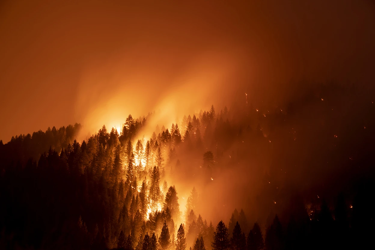
The Dixie wildfire in California this year was the second-largest in state history, and was fuelled by high temperatures and drought. Credit: Eric Thayer/Bloomberg/Getty https://www.nature.com/articles/d41586-021-02990-w
As a leading climate scientist, Paola Arias doesn’t need to look far to see the world changing. Shifting rain patterns threaten water supplies in her home city of Medellín, Colombia, while rising sea levels endanger the country’s coastline. She isn’t confident that international leaders will slow global warming or that her own government can handle the expected fallout, such as mass migrations and civil unrest over rising inequality. With such an uncertain future, she thought hard several years ago about whether to have children.
Dott. Alessio Brancaccio, tecnico ambientale Università degli Studi di L’Aquila, ideologo e consulente tecnico movimento ambientalista Ultima Generazione A22 Network e membro attivo della Fondazione Michele Scarponi Onlus
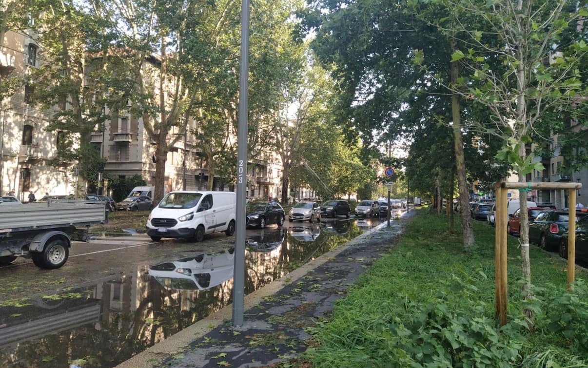
Un violento temporale si è abbattuto – nella notte tra il 24 e il 25 luglio – sul capoluogo lombardo, con forte vento e grandine. Centinaia le segnalazioni di disagi ricevute dai Vigili del Fuoco, tra allagamenti e tetti scoperchiati. Molti gli alberi sradicati da terra in giro per la città, con conseguenti complicazioni per la circolazione di tram e filobus. La Regione Lombardia ha formalizzato la richiesta del riconoscimento dello stato di emergenza
Forti raffiche di vento, fulmini e grandine: un violento temporale si è abbattuto su Milano nella notte tra il 24 e il 25 luglio. Circa 200 le chiamate ricevute dai Vigili del Fuoco, che hanno parlato di una situazione “tragica”. Disservizi anche al sistema elettrico che, solo in serata, ha ripreso a tornare alla normalità
Il temporale è scoppiato intorno alle 04:00. Le grandi quantità di pioggia e grandine cadute in poco tempo hanno causato danni alle linee dei tram – alcune sono cadute a terra – e disagi alla popolazione: ci sono state segnalazioni di tetti scoperchiati, con conseguenti allagamenti.
L’assessore alla Sicurezza e Protezione Civile del Comune di Milano ha parlato di “pioggia di circa 30mm/h”, con una punta massima di 39mm/h registrata in piazza Sicilia.
“Inferno” e “apocalisse” sono tra le parole che si leggono sui social e che accompagnano le immagini del nubifragio. Alcuni video dei cittadini hanno mostrato l’intensità della pioggia e le forti raffiche di vento orizzontale che hanno sfondato o fatto spalancare le finestre di casa.
“Abbiamo vissuto una notte insonne”, ha detto il sindaco di Milano Giuseppe Sala in un video pubblicato sulle sue pagine social, parlando di un vento che “in città ha superato i 100 chilometri all’ora“.
“Ho visto nella mia vita passare 65 estati e quello che sto vedendo ora non è normale, non possiamo più negarlo, il cambiamento climatico sta modificando la nostra vita. Non possiamo semplicemente fare finta di niente e soprattutto non possiamo non fare nulla. Anche Milano deve fare la sua parte e la farà”, ha concluso Sala.
Atm, l’Azienda trasporti milanesi, ha parlato di “gravi danni anche alla nostra rete elettrica” e di alcuni depositi rimasti “senza corrente, mentre alberi caduti e detriti sulle strade bloccano i normali percorsi delle linee“.
Il temporale ha poi danneggiato diversi dehors di bar e ristoranti, mentre scooter e biciclette sono stati gettati a terra dal vento.
In mattinata si segnalavano possibili ritardi – fino a un’ora – anche per la circolazione ferroviaria sulla linea Milano-Venezia e su quella Torino-Milano.
Alcune tegole del Castello sono cadute a terra dalle merlate a causa dei forti venti. Danni anche nella Sala Viscontea, dove di solito si tengono le mostre temporanee.
Il Comune di Milano ha poi disposto la chiusura di tutti i parchi recintati e ha disposto il divieto di accesso ai parchi non recintati e alle aree alberate aperte.
Il presidente della Regione Lombardia Attilio Fontana ha definito lo scenario “sicuramente grave, nel senso che queste improvvise trombe d’aria sono situazioni che non si sono mai verificate su questo territorio”. Poi ha formalizzato al presidente del Consiglio, Giorgia Meloni, ai ministri competenti e al capo dipartimento della Protezione Civile, Fabrizio Curcio, la richiesta del riconoscimento dello stato di emergenza di rilievo nazionale per la Lombardia. In foto: i danni causati dal maltempo al Palazzo di Giustizia a Milano.
A causa dell’innalzamento del fiume Lambro a Milano è stato chiuso temporaneamente lo svincolo di Lambrate ed è stata effettuata un’evacuazione preventiva della comunità Exodus di don Antonio Mazzi. (Nella foto coperture dei tetti volate in strada in via Cortona).
Nella foto il ponteggio di un palazzo crollato in strada anche sui tralicci dei tram in viale Isonzo.
“L’episodio è il primo della storia di Milano, da quanto si registra, e non è stato solo un forte temporale ma un uragano con venti a 100 chilometri all’ora. In dieci minuti sono caduti 40 millimetri di pioggia e nulla che abbia a che vedere con la manutenzione del verde ha a che fare con quanto accaduto”, ha detto l’assessore Grandi. (Nella foto i resti degli alberi caduti vengono tagliati per liberare la viabilità in viale Argonne a Milano).
“Sono caduti centinaia di alberi sani nei parchi e nelle strade, non alberi malati – ha aggiunto l’assessore – e sono state danneggiate tutte le linee aeree del trasporto pubblico locale, ci sono state case allagate, tetti scoperchiati, abbiamo avuto scuole e nostri edifici del Comune allagati, macchine danneggiate e questo non ha nulla di normale”. (Nella foto i danni del maltempo a Milano in viale Romagna).
I danni su vigneti e vivai sono stati ingenti, tanto che la Regione, dopo averli quantificati, chiederà anche lo stato di calamità oltre a una deroga alla legge che esclude dai ristori le aziende non previste di assicurazioni contro le calamità. (Nella foto i danni del maltempo in viale Romagna a Milano).
I danni del maltempo a Milano: in viale Romagna alberi caduti.
I danni del maltempo a Milano: in viale Romagna alberi caduti.
I danni del maltempo a Milano: in viale Romagna alberi caduti.
Da giorni ormai la Lombardia continua a dover fare i conti con il maltempo. Solo pochi giorni fa una tromba d’aria si era abbattuta su Gorgonzola, hinterland milanese.
Colpite anche le altre città e i loro dintorni, da Monza a Brescia. In foto: Milano.
Il nubifragio della scorsa notte ha colpito anche il Pavese. La zona più coinvolta è stata quella della Lomellina, in particolare nell’area tra Vigevano e Mortara. In foto: Milano.
Dott. Alessio Brancaccio, tecnico ambientale Università degli Studi di L’Aquila, ideologo e consulente tecnico movimento ambientalista Ultima Generazione A22 Network e membro attivo della Fondazione Michele Scarponi Onlus
Nuovo allarme lanciato da Coldiretti e da Consorzi Agrari d’Italia. In un comunicato congiunto in occasione delle ‘Giornate in campo 2023’ si legge che: “Il maltempo in Emilia Romagna ha distrutto un raccolto di grano tenero equivalente alla produzione di 200 milioni di chili di pane”.
Una perdita che ridimensiona le stime sulla produzione nazionale di grano con l’Emilia Romagna, con una superficie agricola di oltre un milione di ettari coltivati, oltre a rappresentare l’8% della superficie agricola italiana, è a tutti gli effetti un distretto cerealicolo di assoluta importanza: su circa 570mila ettari di grano tenero a livello nazionale in Emilia Romagna si stimano quest’anno 160mila ettari seminati, poco meno del 30% dell’intera superficie nazionale.
L’alluvione è costata all’Emilia Romagna un taglio della produzione tra il 12 e il 15% di grano con i danni concentrati tra Forlì, Cesena, Ravenna e Faenza e in parte nel Bolognese e Riminese, secondo il monitoraggio di Coldiretti e Cai – Consorzi Agrari d’Italia.
Il consumo annuo pro-capite di pane si situa, in Italia, su circa 41Kg, un quantitativo inferiore a quello registrato in tutti gli altri principali Paesi europei (Romania 88 kg, Germania 80 Kg, Olanda 57 kg, Polonia 52 Kg, Spagna 47 Kg, Francia 44 Kg, Regno Unito 43 Kg).
Secondo un sondaggio Italmopa, l’84% degli Italiani consuma abitualmente pane, mentre il 16% degli intervistati ha dichiarato di non consumare pane o di consumarlo in modo saltuario. Il principale motivo di esclusione del pane dall’alimentazione è di natura dietetica e salutistica.
Tra coloro che consumano abitualmente pane, quello di farina bianca è consumato dal 72% dei votanti mentre coloro che dichiarano di consumare pane di farine integrali ammontano al 39%, una percentuale in crescita rispetto al recente passato.
Inferiori, sono le percentuali – rispettivamente del 28% e del 24% – di coloro che consumano anche pane di semole di grano duro o di farine multi-cereali. Nei giorni scorsi, sempre Coldiretti, aveva avvertito sulla situazione precaria del comparto ortofrutticolo.
In un processo iniziato da 15 anni si sarebbe persa in Italia una pianta da frutto su 5. La situazione peggiore – sottolinea la Coldiretti – si registra per le nettarine con la scomparsa di quasi la metà delle piante (-45%) come per l’uva da tavola (-43%), per le pere (-34%) ma è anche stata estirpata 1 pianta di pesco su tre (-33%), 1 pianta di mandarino su 5 (-20%) e ben il 16% degli alberi di arance, mentre crescono in controtendenza solo i kiwi (+11%).
Una strage di piante da frutto che sta provocando la desertificazione dei territori nelle regioni italiane con drammatici effetti sui consumi nazionali, economia, lavoro, clima, ambiente e salute degli italiani.
Complessivamente la superficie italiana coltivata a frutta si è ridotta a 516mila ettari con la perdita di oltre centomila ettari rispetto a 15 anni fa con conseguenze sul primato produttivo nazionale in Europa che si estende dai kiwi alle pere, dalle ciliegie alle uve da tavola e alle albicocche.
Fonte: Byoblu, la TV libera dei cittadini canale 262 DTV
Allarme lanciato da @coldiretti e Consorzi Agrari d’Italia. A causa del maltempo in Emilia Romagna sono andati persi raccolti per la produzione di 200 milioni di chili di pane.https://t.co/zihXKgsr1b
Dott. Alessio Brancaccio, tecnico ambientale Università degli Studi di L’Aquila, ideologo e consulente tecnico movimento ambientalista Ultima Generazione A22 Network e membro attivo della Fondazione Michele Scarponi Onlus
280 le frane, 42 comuni sott’acqua, 34mila le utenze senza elettricità. Lugo e Cervia allagati. Il cordoglio del Papa per le vittime
Dai primi di Maggio ad oggi 18 del mese, l’Emilia Romagna è in ginocchio a causa dell’emergenza maltempo che ha portato ad un alluvione di vaste proporzioni a Faenza, Imola, Forlì, Cesena, Ravenna, Lugo e Cervia. Al momento si contano 13 vittime, diversi diversi non ancora quantificati e oltre 20 mila sfollati, un evento catastrofico al pari di un terremoto devastante. Di seguito le immagini ed i video che stanno già facendo il giro d’Italia e che ancora una volta testimoniano la mancanza di pianificazione e prevenzione del territorio da parte delle amministrazioni comunali coinvolte dall’evento. I fondi scarseggiano da anni, in attesa dell’arrivo dei fondi del Piano Nazionale di Ripresa e Resilienza (PNRR) e le attività di manutenzione ordinaria e straordinaria delle strade, dei fiumi e dei tombini sono interrotte da più di 20 anni, gli operatori comunali sono invogliati a lavorare per lo più in ufficio con il sedere al caldo, piuttosto che lavorare in strada a sistemare le strade, i fiumi ed il verde pubblico, poi temporali che scaricano giù l’equivalente della pioggia che dovrebbe cadere in 2-3 mesi, fa il resto. In queste ore in cui ancora è in corso l’emergenza maltempo e molti fiumi stanno esondando in diversi comuni della zona di Ravenna e Faenza, pertanto da ore sono in allerta le squadre di soccorso della Protezione Civile, Vigili del Fuoco, Esercito Italiano, Polizia di Stato, Carabinieri, Guardia di Finanza alla ricerca dei dispersi e la situazione meteorologica nelle prossime ore fino a domenica, non promettono niente di buono in queste zone. Di seguito le prime impressionanti immagini di strutture abitative distrutte e di video speciali girati dagli inviati del programma La Vita in Diretta di Alberto Matano su RaiUno e da altri utenti della rete internet, delineano un quadro della situazione attuale che è sconvolgente: molta gente ha dovuto evacuare dalla propria casa, in molti hanno perso tutto, anni di sacrifici buttati via per una calamità naturale che prima d’ora non si era mai vista di questa portata in Italia, neanche l’alluvione di Firenze del 1966 fu di questa enorme portata, a testimonianza dell’eccezionalità di tale evento calamitoso provocato da un vortice depressionario ciclonico instabile di bassa pressione insistente sull’Italia in questi giorni, che nei prossimi anni saranno sempre più frequenti, alla luce degli attuali cambiamenti climatici, che porteranno il nostro Paese ad essere sempre più caldo ed umido anche nei periodi invernali e primaverili, per cui aumenterà di certo la frequenza di questi cicloni sulla terraferma o i Medicane in mare sul Mediterraneo, per effetto dell’aumento delle temperature a livello globale e locale di 2-2,5°C, che renderanno il nostro Paese sempre più invivibile: nelle grandi città metropolitae andrà considerato anche il problema isole di calore che aumenteranno ulteriormente la temperatura per la presenza di cementificazioni connesse all’ambiente urbano (marciapiedi, spartitraffici, gas di scarico delle automobili a motore termico diesel e benzina, riscaldamenti a gasolio centralizzati, solo per fare alcuni esempi) che porteranno la temperatura nelle città a livelli smepre più critici per un aumento di 5-7°C: città come Roma, Milano e Torino nei prossimi 5-6 anni potrebbero arrivare d’estate a toccare temperature massime di 48-50°C come Marrakech in Marocco, il che è impressionante soltanto a parlarne, figuriamoci a vivere direttamente una situazione del genere. Eccole qui le prime immagini ed i video dell’alluvione di questi giorni in corso in Emilia Romagna.
Alluvione Emilia-Romagna, le vittime salgono a 13. Oltre 10mila sfollati. DIRETTA
Gli sfollati e le persone fatte evacuare sono migliaia. Il 23 maggio si terrà un Cdm sull’emergenza: sarà deliberato lo stato di calamità. Bonaccini: danni per qualche miliardo. Anche per la giornata di oggi resta allerta rossa nella regione, con scuole chiuse fra Cesena e Bologna. Arancione in Lombardia, Marche e Toscana
Dott. Alessio Brancaccio, tecnico ambientale Università degli Studi di L’Aquila, ideologo e consulente tecnico movimento ambientalista Ultima Generazione A22 Network e membro attivo della Fondazione Michele Scarponi Onlus
El Niño, un fenomeno climatico frutto di complesse dinamiche atmosferiche e i cui effetti si ripercuotono in tutto il mondo, sta arrivando. Ad annunciare il suo imminente sviluppo sono stati quelli che vengono considerati i precursori di questo fenomeno, noti come le onde di Kelvin. Infatti, i dati raccolti dal satelliteSentinel-6 Michael Freilich, parte della missione Copernicus Sentinel-6/Jason-CS, mostrano come le onde di kelvin sono alte circa 5-10 centimetri sulla superficie dell’oceano Pacifico e lunghe centinaia di chilometri, e si stanno muovendo da ovest a est lungo l’equatore verso la costa occidentale del Sud America.
Ricordiamo brevemente che El Niño è un fenomeno climatico periodico (ogni 5 anni circa) che può influenzare i modelli meteorologici in tutto il mondo e che comporta un riscaldamento della superficie del Pacifico. Associato all’indebolimento degli alisei (i venti che soffiano da est a ovest), infatti, El Niño è caratterizzato da livelli del mare più alti e temperature degli oceani più calde della media. In particolare, gli esperti sanno che una serie di onde di Kelvin, onde che si formano all’Equatore e portano acqua calda, che iniziano nella stagione primaverile è un precursore dell’arrivo di un El Niño. Come ricorda la Nasa, l’acqua si espande man mano che si riscalda, quindi i livelli del mare tendono ad essere più alti nei luoghi con acqua più calda.
NASA/JPL-Caltech
La rilevazione
Grazie all’altimetro radar, strumento fornito dal Jet Propulsion Laboratory della Nasa che utilizza segnali a microonde per misurare l’altezza della superficie dell’oceano, Sentinel-6 Michael Freilich ha rilevato che entro la fine di aprile le onde di Kelvin hanno accumulato acqua più calda e livelli del mare più alti (indicati nell’immagine in rosso e bianco) al largo delle coste di Perù, Ecuador e Colombia. “Guarderemo questo El Niño come un falco”, ha commentato Josh Willis, scienziato del progetto Sentinel-6 Michael Freilich presso il Jpl. “Se sarà potente, il mondo vedrà un riscaldamento record, ma qui nel sud-ovest degli Stati Uniti potremmo assistere a un altro inverno umido, proprio sulla scia di quello che abbiamo avuto lo scorso inverno”.
Di recente, inoltre, anche la statunitense National Oceanographic for Air Administration (NOAA) sia la World Meteorological Organization (WMO, l’Organizzazione meteorologica mondiale) hanno lanciato l’allerta dell’arrivo de El Niño, prevedendo maggiori possibilità che si sviluppi entro la fine dell’estate. Il monitoraggio continuo delle condizioni oceaniche nel Pacifico da parte di strumenti e satelliti come Sentinel-6 Michael Freilich dovrebbe aiutare a chiarire nei prossimi mesi quanto forte potrebbe diventare. “Quando misuriamo il livello del mare dallo Spazio utilizzando altimetri satellitari, conosciamo non solo la forma e l’altezza dell’acqua, ma anche il suo movimento, come le onde di Kelvin e altre onde”, ha spiegato Nadya Vinogradova Shiffer, esperta della Nasa e manager di Sentinel-6 Michael Freilich. “Le onde dell’oceano diffondono calore intorno al pianeta, portando calore e umidità sulle nostre coste e cambiando il nostro clima”.
Dott. Alessio Brancaccio, tecnico ambientale Università degli Studi di L’Aquila, ideologo e consulente tecnico movimento ambientalista Ultima Generazione A22 Network e membro attivo della Fondazione Michele Scarponi Onlus
Il mondo deve prepararsi per una calda corrente di El Niño, che quest’anno farà aumentare le temperature a livelli record: le possibilità raggiungeranno il 60% da maggio a luglio e poi aumenterà al 70% tra giugno e agosto e all’80% tra luglio e settembre, ha affermato oggi a Ginevra l’Organizzazione meteorologica mondiale (Wmo). “Lo sviluppo di un El Niño porterà molto probabilmente a un nuovo picco nel riscaldamento globale e aumenterà la possibilità di battere i record di temperatura”, ha affermato Petteri Taalas, capo dell’Organizzazione meteorologica mondiale delle Nazioni Unite.
El Niño è un fenomeno climatico di riscaldamento del Pacifico tropicale centrale e orientale, fino alle coste di Peru ed Ecuador. Si ripete con intervalli da 2 a 7 anni e dura da 9 a 12 mesi. Porta ondate di calore, siccità e alluvioni in varie parti del mondo. In particolare, piogge su parti del Sudamerica, nel sud degli Stati Uniti, nel Corno d’Africa e nell’Asia centrale, e siccità sull’Australia, l’Indonesia e parti dell’Asia meridionale. El Niño d’estate alimenta gli uragani nel Pacifico centro-orientale e li ostacola sull’Atlantico.
Il fenomeno opposto, chiamato La Niña, consiste nel raffreddamento della stessa area del Pacifico tropicale centrale e orientale. Negli ultimi tre anni la Niña si è ripetuta costantemente. Secondo l’Organizzazione meteorologica mondiale, l’anno più caldo da quando ci sono rilevazioni scientifiche, il 2016, è stato così per l’effetto combinato di un Niño molto potente e del riscaldamento globale di origine umana.
“Il mondo dovrebbe prepararsi allo sviluppo del Nino – avverte Taalas -. Potrebbe portare sollievo dalla siccità nel Corno d’Africa, ma potrebbe anche scatenare più eventi meteorologici estremi. Questo sottolinea la necessità dell’iniziativa lanciata dall’Onu ‘Primo allarme per tutti’, per istituire in tutti i paesi del mondo sistemi di allarme tempestivi per gli eventi eccezionali”.
Dott. Alessio Brancaccio, tecnico ambientale Università degli Studi di L’Aquila, ideologo e consulente tecnico movimento ambientalista Ultima Generazione A22 Network e membro attivo della Fondazione Michele Scarponi Onlus
Apprendere di più in merito questi Fiumi nel Cielo
AGGIORNAMENTO: 31 Marzo, 2023. Aggiornamento riguardo il fare una dichiarazione chiarificatrice nel testo introduttivo
I fiumi atmosferici sono regioni relativamente lunghe e strette nell'atmosfera, come i fiumi nel cielo, che trasportano la maggior parte del vapore acqueo al di fuori dei tropici. Mentre i fiumi atmosferici possono variare notevolmente in termini di dimensioni e forza, il fiume atmosferico medio trasporta una quantità di vapore acqueo approssimativamente equivalente al flusso medio di acqua alla foce del fiume Mississippi. Fiumi atmosferici eccezionalmente forti possono trasportare fino a 15 volte quella quantità. Quando i fiumi atmosferici approdano, spesso rilasciano questo vapore acqueo sotto forma di pioggia o neve.
Anche se i fiumi atmosferici sono disponibili in molte forme e dimensioni, quelli che contengono le maggiori quantità di vapore acqueo e i venti più forti possono creare precipitazioni estreme e inondazioni, spesso bloccandosi su bacini idrografici vulnerabili alle inondazioni. Questi eventi possono interrompere il viaggio, provocare smottamenti e causare danni catastrofici alla vita e alla proprietà. Un esempio ben noto è il "Pineapple Express", un forte fiume atmosferico che è in grado di portare l'umidità dai tropici vicino alle Hawaii alla costa occidentale degli Stati Uniti.
Non tutti i fiumi atmosferici causano danni; la maggior parte sono sistemi deboli che spesso forniscono benefiche piogge o nevicate che sono cruciali per l'approvvigionamento idrico. I fiumi atmosferici sono una caratteristica chiave nel ciclo globale dell'acqua e sono strettamente legati sia all'approvvigionamento idrico che ai rischi di alluvione, in particolare negli Stati Uniti occidentali.

Mentre i fiumi atmosferici sono responsabili di grandi quantità di pioggia che possono produrre inondazioni, contribuiscono anche a un benefico aumento del manto nevoso. Una serie di fiumi atmosferici ha alimentato le forti tempeste invernali che hanno colpito la costa occidentale degli Stati Uniti da Washington occidentale alla California meridionale dal 10 al 22 dicembre 2010, producendo da 11 a 25 pollici di pioggia in alcune aree. Questi fiumi hanno anche contribuito al manto nevoso nelle Sierras, che hanno ricevuto il 75% della sua neve annuale entro il 22 dicembre, il primo giorno intero dell'inverno.

La ricerca NOAA (ad esempio, NOAA Hydrometeorological Testbed e CalWater) utilizza satelliti, radar, aerei e altre osservazioni, oltre a importanti miglioramenti del modello meteorologico numerico, per comprendere meglio i fiumi atmosferici e la loro importanza sia per il meteo che per il clima.

La ricerca scientifica fornisce dati importanti che aiutano i meteorologi del Servizio Meteorologico Nazionale del NOAA a emettere avvisi per potenziali forti piogge e inondazioni in aree soggette agli impatti dei fiumi atmosferici con un anticipo di cinque o sette giorni.

Pineapple Express

Un forte fiume atmosferico che è in grado di portare l'umidità dai tropici vicino alle Hawaii alla costa occidentale degli Stati Uniti.

Scopri di più su come NOAA studia i fiumi atmosferici e monitora le attuali condizioni atmosferiche del fiume.

Ultimo aggiornamento: Marzo 2023
Istituto di Scienze dell’Atmosfera e del Clima (ISAC)
Atmospheric River nel Mediterraneo
L’articolo pubblicato sul Monthly Weather Review, scritto dai ricercatori CNR-ISAC Silvio Davolio, Mario Miglietta, Sante Laviola e Vincenzo Levizzani assieme a Stefano Della Fera dell’Università di Bologna, descrive i meccanismi responsabili delle intense precipitazioni che hanno colpito l’Italia a fine di Ottobre 2018, associate alla tempesta Vaia. Lo studio evidenzia la presenza ed il ruolo determinante di un Atmospheric River nel Mediterraneo, ovvero di un trasporto cospicuo di vapore acqueo dalle regioni tropicali organizzato lungo uno stretto corridoio che ha attraversato il continente Africano, nell’alimentare le intense precipitazioni sulla penisola.
Dott. Alessio Brancaccio, tecnico ambientale Università degli Studi di L’Aquila, ideologo e consulente tecnico movimento ambientalista Ultima Generazione A22 Network e membro attivo della Fondazione Michele Scarponi Onlus